GRAVITY GOODS ROPEWAY
Hence y = 4bx2 + (h-4b)x
l2 l
(i)
This is equivalent to the parabolic equation,
y = ax2 + bx
(ii)
Hence from this relation, y for each corresponding
x is obtained and the rope curve can be plotted.
Integrating the equation (ii),
dy
dx
= Tan (β) = 2ax + b
(iii)
This relation gives the slope of the curve at the
point of consideration. Hence, we can obtain the
tension in the rope anywhere from the following
relation,
T = H / Cos (β)
The curve of the rope can be obtained from the
following relation too.
T
Hβ
w
w
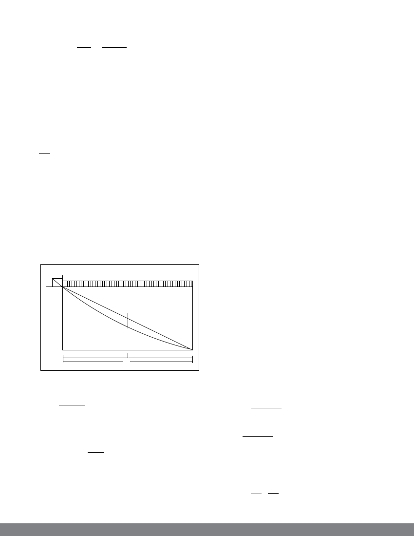
bx
Figure 15
x
I
I-x
When the chord is horizontal, we know that,
b = w (l-x) x
(i)
2H
And the rope sag is maximum at x = l/2
So, bmax =
wl2
8H
(ii)
Now dividing equation (i) by (ii), we obtain the
ratio
18
b: bmax = 4.x (1- x )
ll
(iii)
As the maximum sag is known, the rope curve can
be plotted from this relation.
The curve shape calculation using the catenary’s
equation is elaborative and arduous. The errors
arising from the approximation when replacing
the catenary by parabola do not exceed 2.6 per
cent. Therefore, in almost all the cases, it can be
assumed with sufficient accuracy that the rope
curve is parabolic. For small span and sag, the
error due to the assumption amounts to fraction
of one per cent. The error varies proportionately
with the ratio of b/l.
With uniformly distributed load over the rope span
in the plan view, the error amounts to:
b/l < 1/20
b/l = 1/10
b/l =1/5
error < 0.3%
error = 1.3%
error = 5%
Some codes for aerial ropeway suggest that the
profile of the rope may be considered parabolic if
the sag is less than 10 per cent of the span.
B) Rope curve under single moving load
The total rope sag will be equal to the sum of the
sag due to the own weight of the rope and the
weight of the trolley W.
Hence, btotal = b1 + b2 where b1 and b2 are the
rope sags due to the self weight of the rope and
the imposed load respectively at the point of
consideration in the rope profile
And b1 = w x (l-x)
2H
b2 = W (l – x )
H
The sag would be maximum, at x = l/2
Hence
bmax =
l2 (w + 2W )
8H l